Contents
Linear regression
Create a figure with white background
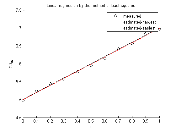
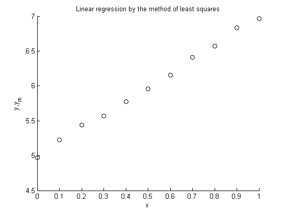
h=figure;
set(h,'Color','w')
hold all
title('Linear regression by the method of least squares')
xlabel('x');
ylabel('y,y_m')
Measured values
Here the "measured" values are determined artificially using the function 2x+5 and introducing some randomnes for simulation of the measurement error.
x=0:0.1:1;
N=length(x);
ym=2*x+5*ones(size(x))+0.1*rand(size(x))-0.05*ones(size(x));
% Plot the measured values using circles
plot(x,ym,'ok')
Calculate the ecuation of the best fitting line using the method of
least squares
First the 'hardest way'
sumx=sum(x);
sumx2=sum(x.^2);
sumym=sum(ym);
sumxym=sum(x.*ym);
C=[sumx2 sumx; sumx N];
D=[sumxym; sumym];
% The solution of a linear equation system can be calculated in two ways:
% First: A=C\D;
% Second:
A=inv(C)*D;
% Now the vector 'A' contains the parameters of the best fitting line.
% Calculate the points of the line and plot the line.
y=polyval(a,x);
plot(x,y,'-k');
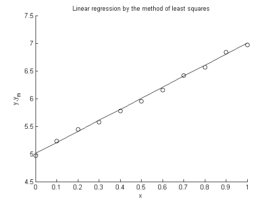
Using polyfit
Secondly the easiest way
a=polyfit(x,ym,1);
% Now the vector 'a' contains the parameters of the best fitting line.
% Calculate the points of the line and plot the line.
y=polyval(a,x);
plot(x,y,'-r');
legend('measured','estimated-hardest','estimated-easiest')